Seattle, located in the Pacific Northwest region of the United States, is a bustling city with
a diverse population and a reputation for being one of the most liveable cities in the
country. However, like any major metropolitan area, Seattle is not immune to crime.
In this Hackathon our team intends to inform the public about which areas are the most crime
ridden, provide valuable insights to explain these occurances, and use machine learning to
predict crime rates.
Crime in downtown Seattle has a significant impact on the public, including residents,
workers, and visitors to the area. The high rate of property crimes, such as theft and
burglary, can make people feel unsafe and lead to a loss of trust in the community.
In addition, the increase in violent crimes, such as assault and homicide, can cause fear and
anxiety, especially for those who frequent downtown areas at night. Businesses in the area may
also be affected, as customers may be hesitant to visit and spend money in areas where they
feel unsafe.
The city of Seattle has implemented various measures to address the issue, including increased
police presence and community outreach programs, but there is still much work to be done to
ensure the safety and security of the downtown area.
Theft/Larceny Dominates All Crimes
While crime in downtown Seattle may receive more attention due to its higher concentration of businesses and visitors, it is important to note that all neighborhoods in the city are experiencing similar problems with crime. Property crimes such as car theft and break-ins, as well as violent crimes like domestic violence and robbery, are prevalent in many Seattle neighborhoods. These crimes can have a significant impact on the well-being of residents and lead to a loss of trust in the community. We noticed that the vast majority of crime is Larceny/Theft realted incidents, followed by Assault and then Burglary/Breaking and Entering.
Addressing crime in all neighborhoods is a critical issue for the city, and requires a collaborative effort from law enforcement, community organizations, and residents alike.
We have created an overall crime index and a night crime index. Overall crime index is
calculated as the ratio of crime counts for that neighborhood (MCPP) divided by the average
crime count for all of Seattle. This means that if the overall crime index is around one, the
overall crime in that neighborhood is aroudn the average for Seattle. If the crime index is
two, it’s twice as much! Downtown Commerical has ~3.7 crime index! Other downtown areas (Queen
Anne and Capitol Hill) are also above 3, indicating these areas are crime hotspots.
We created a night time modifier as well. We first divided the total night time counts for
each neighborhood and divided by the average for all of Seattle and then subtracted one. This
modifier gives us an idea of how dangerous an area is compared to an average Seattle
neighborhood. If the modifier is positive, the neighborhood is more dangerous. The more
positve, the higher the crime rate at night compared to the rest of Seattle. Conversely, if
the night index is negative, the area is more safe at night compared to Seattle’s nights
(doesn’t necessarily mean it is more safe than in the day).
Finally, we created a night index which is a sum of both of these values. This gives us an
index of how much crime happens at night overall compared to the rest of Seattle (similar to
the overall crime index, but specifically for night).
*One intersting data point we saw was that the night modifier for the downtown commercial
index was negative even though it had the highest overall crime index. We predict this is
because all the businesses are closed at this time and thus there’s less foot traffic.
**We define night as after 6 PM and before 7 AM
Machine Learning
We want to make a machine learning model to predict the number of crimes for any given Parent
Offense per day. We did the same pre-processing as above where we removed all the data like
so:
df = pd.read_csv('/workspaces/Datathon2023/dataset/SPD_Crime_Data__2008-Present.csv')
#make offense start date time a datetime object
date_time = pd.to_datetime(df['Offense Start DateTime'], format='%m/%d/%Y %H:%M:%S %p')
df['start_date_time'] = date_time

#only keep the rows that have a offense start date more than 2008
df = df[df['start_date_time'] >= '2008-01-01']
We further grouped together the dataset to find the number of occurrences of any given parent
group per day:
df = df.set_index('start_date_time')
df = df.groupby([pd.Grouper(freq='D'), 'Offense Parent Group']).size().reset_index(name='Count')
Then, we segmented based on the Offense Parent Group. For the sake of this report, we’ll use
Larceny-Theft as our Parent Group (this group had the largest number of samples), but we
performed the same process on all the groups. After segmenting, we split our data into train,
validation, and test with a 70-20-10 split.
df_model = df[df['Offense Parent Group'] == OFFENSE_PARENT_GROUP]

#drop all columns except for date and count
df_model = df_model.drop(columns=['Offense Parent Group'])

n = len(df_model)
train_df = df_model[0:int(n*0.7)]
val_df = df_model[int(n*0.7):int(n*0.9)]
test_df = df_model[int(n*0.9):]

num_features = df_model.shape[1]
We then normalized the number of crimes per day by subtracting the mean and then dividing by
the standard deviation. We made sure to use the mean and standard deviation for only the train
dataset since the model should be blind to the validation and test datasets.
#normalize the data for the Count column
train_mean = train_df['Count'].mean()
train_std = train_df['Count'].std()

train_df['Count'] = (train_df['Count'] - train_mean) / train_std
val_df['Count'] = (val_df['Count'] - train_mean) / train_std
test_df['Count'] = (test_df['Count'] - train_mean) / train_std

#make the date column the index
train_df = train_df.set_index('start_date_time')
val_df = val_df.set_index('start_date_time')
test_df = test_df.set_index('start_date_time')
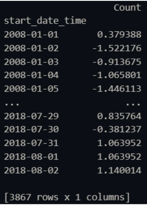
Our final datasets ended up looking like this (train dataset for the Larceny-Theft Parent
Group pictured below)
Baseline Model
The first model we made acted as a naive baseline. The model simply says that tomorrow’s
crime count will be the same as today’s. Here’s how well it fits on our dataset (split into
the first three predictions)
We can see that the data follows the trend, but obviously it lags behind. Furthermore, this
model would be horrible at predicting the future with unknown data. However, it gives us a
good baseline as we have high variability in our dataset (almost like a stock market) and the
naive baseline oftentimes outperforms many complex models in market scenarios. Our mean
absolute error, in this case, is 0.8533. Not bad, but it can be improved. Time for some
machine learning! We elected to use Tensorflow in making our models.
Linear Model
The simplest model we can make while still learning to fit our data is a linear model. In
TensorFlow, this is just one Dense block.
linear = tf.keras.Sequential([
tf.keras.layers.Dense(units=1)
])
Our loss in this case is Mean Squared Error, while we use the Adam optimizer. Let’s take a
look at how this simplistic model performs:
It looks like it’s better! The prdedictions are much closer to the labels than in our baseline
case which is promising! Our mean absolute error in this case is 0.7216, we’re getting better.
Let’s make our model more complex.
Multiple Step Inputs
So far, all of our methods have used the previous time step in order to predict the next one.
Intuitively, we would want our model to be able to look at historical data as well so that it
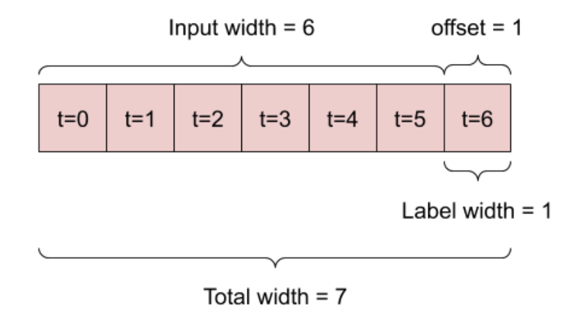
can better predict what will happen in the future. How can we do this? Let’s say we want to
predict one day in the future passing in a week’s worth of data. We can use a technique called
Data Windowing to do this. We take the first 7 points in our dataset as our input, and then
use the 8th point as our label. Then we move our window over by one and take days 2-8 as our
input, and have the 9th day as our label. Move throughout the entirety of the dataset using
this approach and you have yourself a windowed dataset! Here’s a diagram from Tensorflow’s API
to help explain this concept:
Let’s use this new dataset coupled with adding more dense blocks to our linear model to make a
deep neural network!
multi_step_dense = tf.keras.Sequential([
tf.keras.layers.Flatten(),
tf.keras.layers.Dense(units=32, activation='relu'),
tf.keras.layers.Dense(units=32, activation='relu'),
tf.keras.layers.Dense(units=32, activation='relu'),
tf.keras.layers.Dense(units=32, activation='relu'),
tf.keras.layers.Dense(units=1),
tf.keras.layers.Reshape([1, -1]),
])

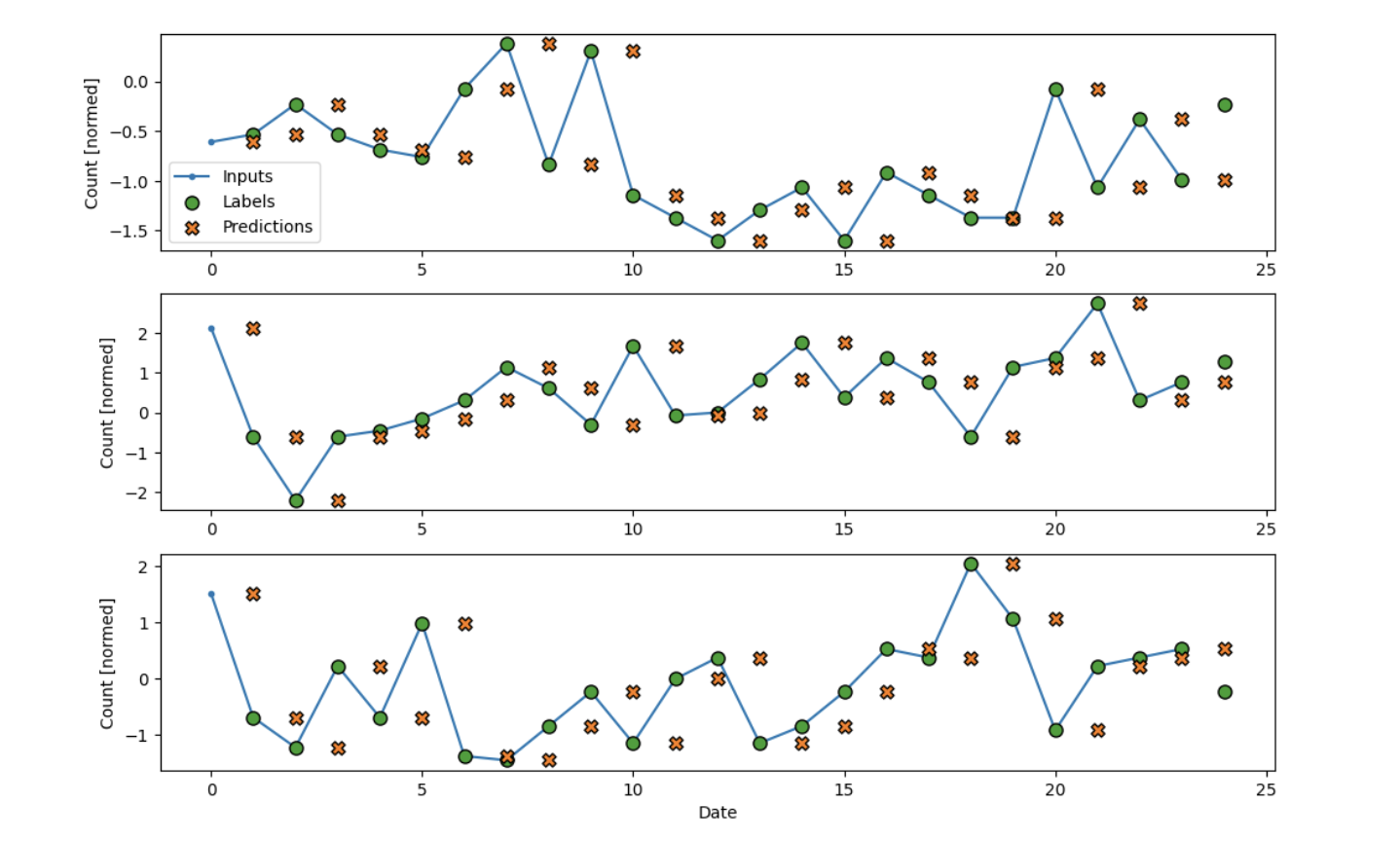
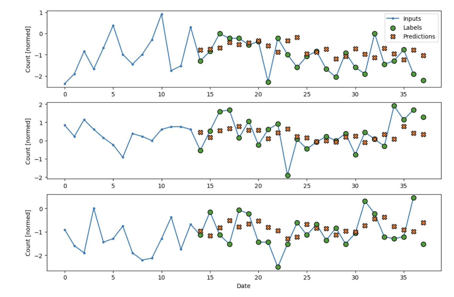
It seems to fit really well for the first couple data points! It struggled with the middle
case where there was high fluctuation in the actual label, but it found the trend for the
other two almost perfectly. Our mean average error in this case is only 0.66! Let’s try some
other methods and see if we can do even better
Convolutional Neural Netowork
Generally used in image processing, convolutional neural networks apply a convolution on top
of the input data. It allows us to pool together our input data, so that we can pass in
multiple lengths on inputs.
conv_model = tf.keras.Sequential([
tf.keras.layers.Conv1D(filters=32,
kernel_size=(CONV_WIDTH,),
activation='relu'),
tf.keras.layers.Dense(units=32, activation='relu'),
tf.keras.layers.Dense(units=16, activation='relu'),
tf.keras.layers.Dense(units=1),
])
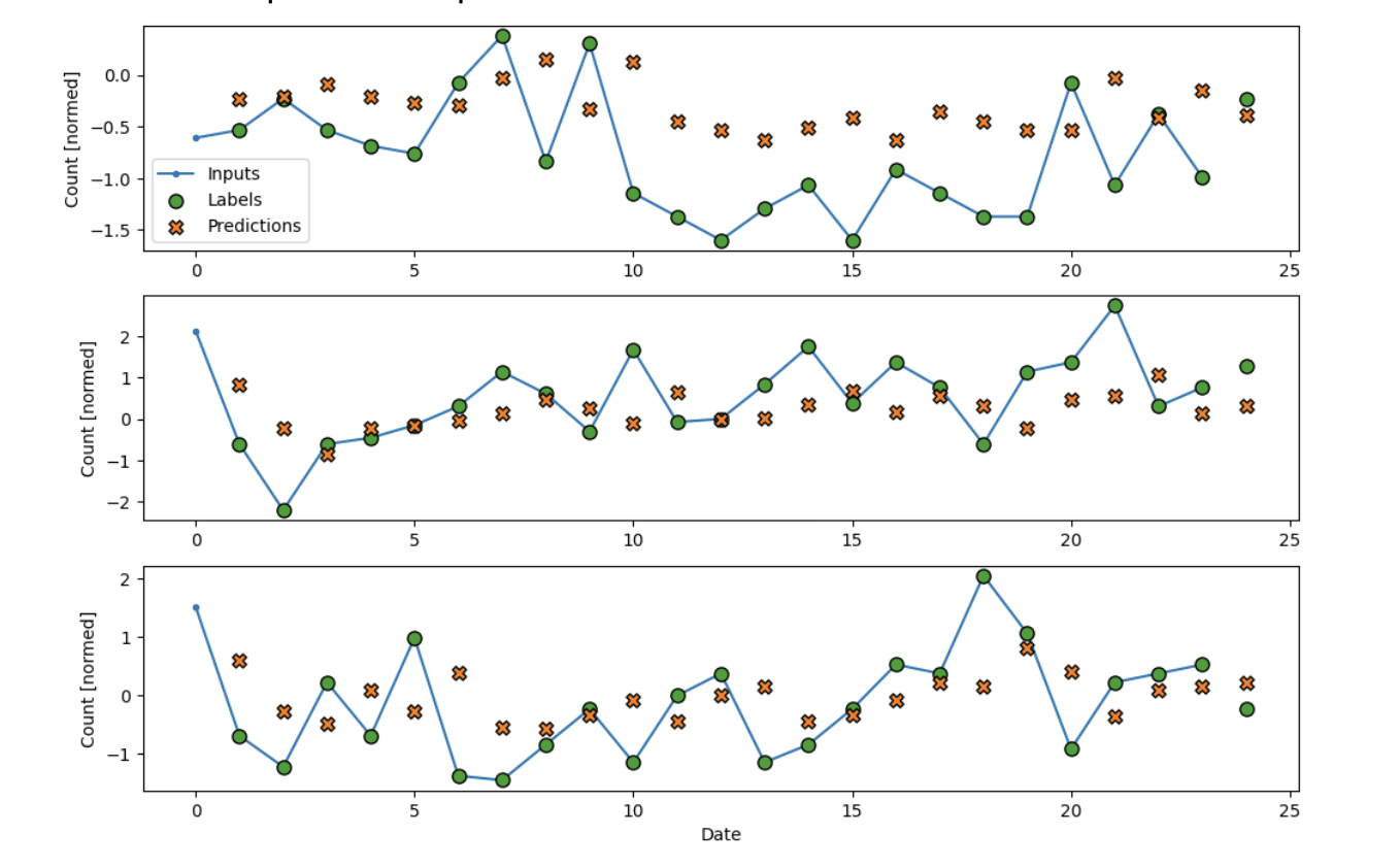
We see a very good fit on our data! Other than wild fluctuations, our CNN seems to be sticking
very closely with the actual predictions. Mean average error in this case is 0.66.
Long Short-Term Memory (LSTM)
Recurrent Neural Networks use Long Short-Term Memory Layers. These keep an internal state
through the time steps, having a “memory” of sorts while going through the layers. As a
result, they work really well for time series data
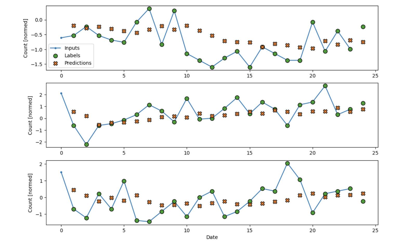
In the cases without fluctuation, the RNN seems to fit a little bit better than the other
models. It sticks very close to the trend line. The mean average error in this case is 0.65.
So, the overall performance of our models looks like so:
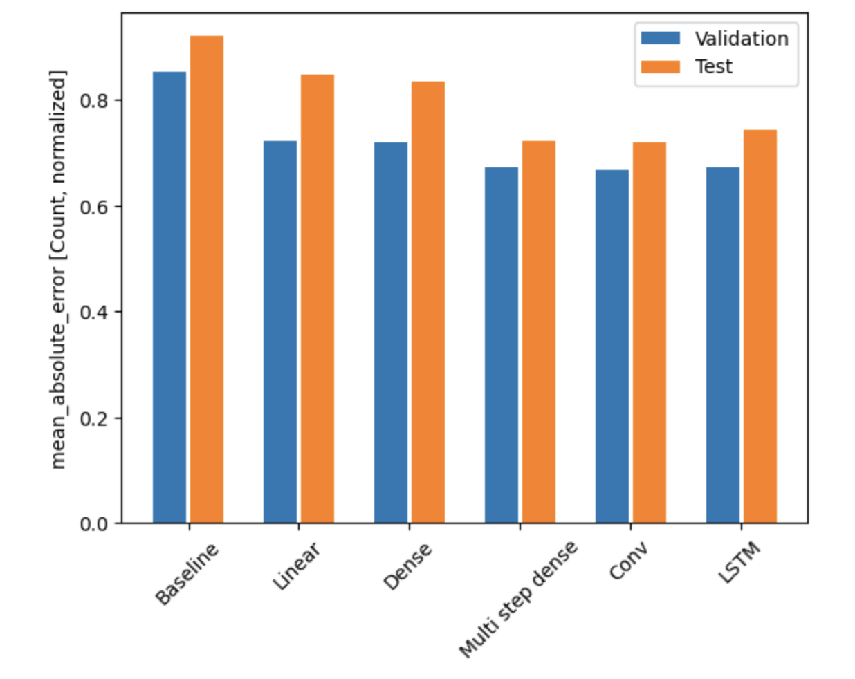
We showed a model can learn pretty well! Other than on the large day-by-day changes, the model
is able to fit to the data quite nicely. The best model in this case (looking at the test
data) seems to be the CNN, followed by the multi-step dense network, then the LSTM. With a
mean average error of just 0.65, we are able to predict the number of cases to a high
accuracy. This means that with a mean of about 70 cases per day for larceny-theft, our model
is able to come within 8 cases of the true label in our predictions.
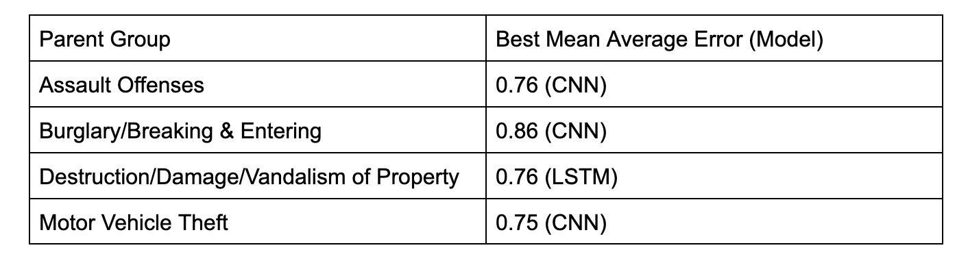
Other Parent Groups
Here are the values for the next 4 most common Parent Groups